Introduction
Let's say you have a worksheet with thousands of rows of data. It would be extremely difficult to see patterns and trends just from examining the raw information. Similar to charts and sparklines, conditional formatting provides another way to visualize data and make worksheets easier to understand.
Optional: Download our practice workbook.
Watch the video below to learn more about conditional formatting in Excel.
Understanding conditional formatting
Conditional formatting allows you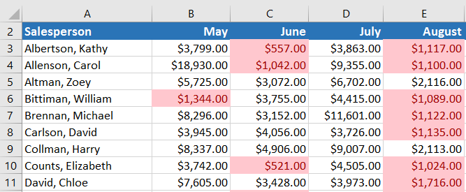
To create a conditional formatting rule:
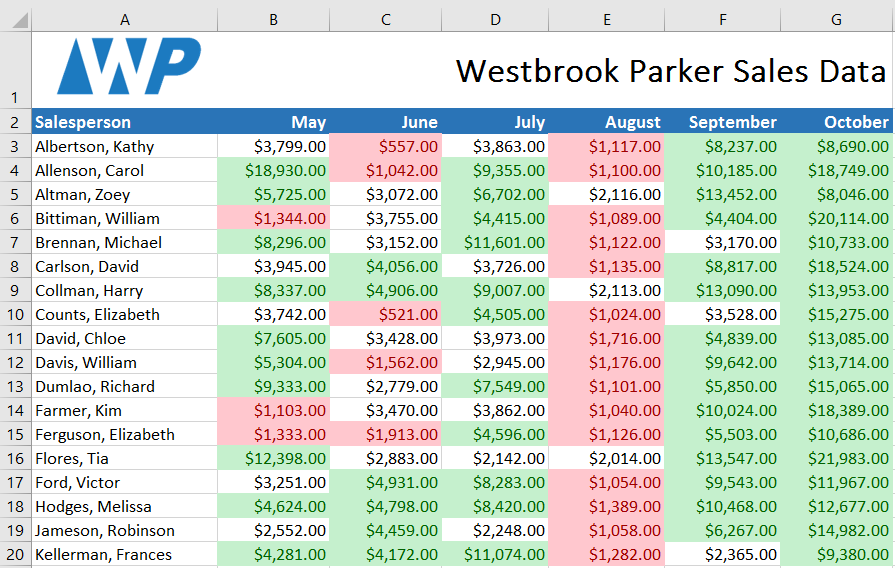
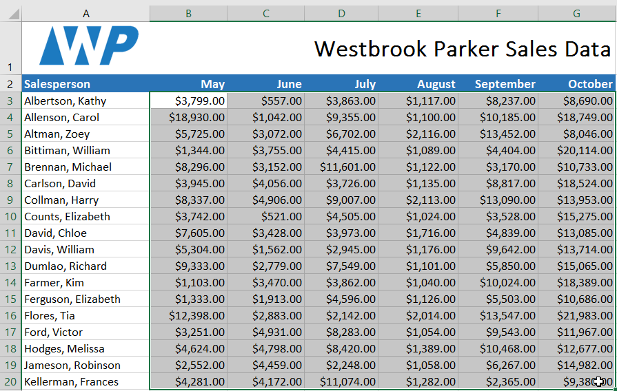
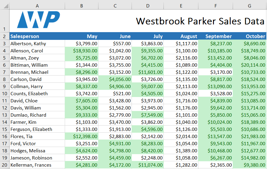
In our example, we have a worksheet containing sales data, and we'd like to see which salespeople are meeting their monthly sales goals. The sales goal is $4000 per month, so we'll create a conditional formatting rule for any cells containing a value higher than 4000.- Select the desired cells for the conditional formatting rule.
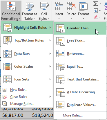
- From the Home tab, click the Conditional Formatting command. A drop-down menu will appear.
- Hover the mouse over the desired conditional formatting type, then select the desired rule from the menu that appears. In our example, we want to highlight cells that are greater than $4000.
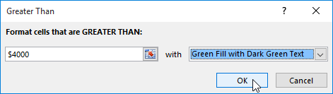
- A dialog box will appear. Enter the desired value
( - Select a formatting style from the drop-down menu. In our example, we'll choose Green Fill with Dark Green Text, then click OK.
- The conditional formatting will be applied to the selected cells. In our example, it's easy to see which salespeople reached the $4000 sales goal for each month.
You can apply multiple conditional formatting rules to a cell range or worksheet, allowing you to visualize different trends and patterns in your data.